Chronic Kidney Disease

Classification of chronic kidney disease

Table of Contents

1. Project Overview.
2. Problem Statement.
3. Metrics.
4. Data Exploration and visualization.
5. Methodology.
6. Results.
7. Conclusion.
8. Licensing, Authors, Acknowledgements.

1. Project Overview

This article is for my Udacity Data Science Nanodegree capstone project and uses a dataset on chronic kidney disease from Kaggle. Predictions have been made on patients’ kidney data to determine whether there are any clear indications of chronic kidney disease.

2. Problem Statement

A few years ago during pregnancy I was placed in the high risk group due to raised blood pressure (gestational hypertension). Ten days after birth my blood pressure rose even higher and it was determined to be preeclampsia; pronounced [pree·uh·klamp·see·uh]. Left untreated preeclampsia can lead to organ failure; in particular to the liver and kidneys.

This data science project will be to investigate kidney data (described in the Kaggle link above) to predict whether or not a patient has chronic kidney disease. The expectation is that the results of this project could be used to benefit people who have had their blood taken in hospital; features of their blood could be used in a model to identify chronic kidney disease which may not have been previously picked up. If I knew my equivalent data I could predict my likelihood of having this disease since having preeclampsia years ago.

Questions to be answered

1. Can we predict chronic kidney disease from the features in the dataset?
2. Which features are key to the predictions?
3. Which is the best model to use and why?

3. Metrics.

A few models will be tried, starting with logistic regression since it is used to explain the relationship between one dependent binary variable (disease present or not) and one or more nominal, ordinal, interval or ratio-level independent variables. The metrics used to measure the performance of the models will be predictions on the test data, score/classification accuracy, and confusion matrices.

The data has been prepared into train and test files and a set of data models have been used in the predictions after a series of feature engineering steps.

The columns and their descriptions are as follows:

1. age - age: Age(numerical) - in years
2. bp - blood pressure: Blood Pressure(numerical) - in mm/Hg
3. sg - specific gravity Specific Gravity(nominal) - (1.005,1.010,1.015,1.020,1.025)
4. al - albumin Albumin(nominal) - (0,1,2,3,4,5)
5. su - sugar Sugar(nominal) - (0,1,2,3,4,5)
6. rbc - red blood cells Red Blood Cells(nominal) - (normal,abnormal)
7. pc - pus cell Pus Cell (nominal) - (normal,abnormal)
8. pcc - pus cell clumps Pus Cell clumps(nominal) - (present,notpresent)
9. ba - bacteria Bacteria(nominal) - (present,notpresent)
10. bgr - blood glucose random Blood Glucose Random(numerical) - in mgs/dl
11. bu - blood urea Blood Urea(numerical) - in mgs/dl
12. sc - serum creatinine Serum Creatinine(numerical) - in mgs/dl
13. sod - sodium Sodium(numerical) - in mEq/L
14. pot - potassium Potassium(numerical) - in mEq/L
15. hemo - hemoglobin Hemoglobin(numerical) - in gms
16. pcv - packed cell volume Packed Cell Volume(numerical)
17. wc - white blood cell count White Blood Cell Count(numerical) - in cells/cumm
18. rc - red blood cell count Red Blood Cell Count(numerical) - in millions/cmm
19. htn - hypertension Hypertension(nominal) - (yes,no)
20. dm - diabetes mellitus Diabetes Mellitus(nominal) - (yes,no)
21. cad - coronary artery disease Coronary Artery Disease(nominal) - (yes,no)
22. appet - appetite Appetite(nominal) - (good,poor)
23. pe - pedal edema Pedal Edema(nominal) - (yes,no)
24. ane - anemia Anemia(nominal) - (yes,no)
25. Our target: class - Class (nominal)- class - (ckd,notckd)

4. Data Exploration and visualization.

How To Interact With The Project

Install Jupyter notebook and open the .ipynb file to run the cells within it. After feature engineering the following models were applied and the resulting accuracy/scores and confusion matrices calculated.

File Descriptions

1. CKD Prediction.ipynb: Jupyter notebook with a step-by-step analysis of kidney data to predict chronic kidney disease.
2. kidney_disease_train.csv: messages created by thepublic in the native language, converted into english.
3. kidney_disease_test.csv: categories into which messages fall; water, medical, etc.
4. kidney_failure.jpg: a drawing of a funtioning kidney and a failed kidney.

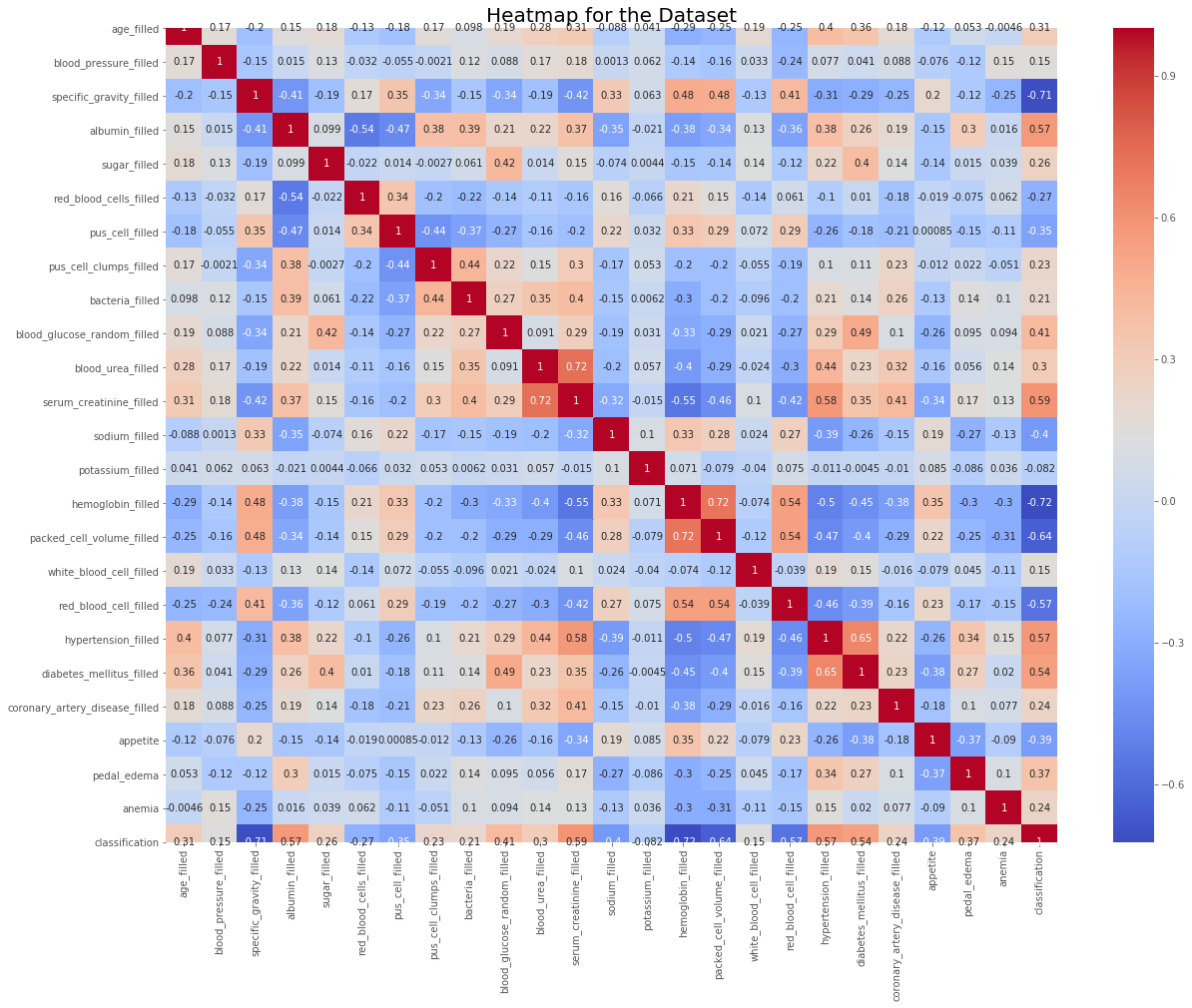
The heatmap below shows the relationships between features and the target (‘classification’). The features ‘packed cell volume’ and ‘hemoglobin’ mostly correlate with each other, and the feature ‘serum creatine’ most positively correlates with having chronic kidney disease.

Packed cell volume is the the volume percentage of red blood cells in blood. Hemoglobin is a protein in your red blood cells that carries oxygen to your organs and tissues and transports carbon dioxide from your organs and tissues back to your lungs. Low hemoglobin levels means you have a low red blood cell count (anemia).

It makes sense that these show correlation as they both refer to the number of red blood cells in the blood.

---

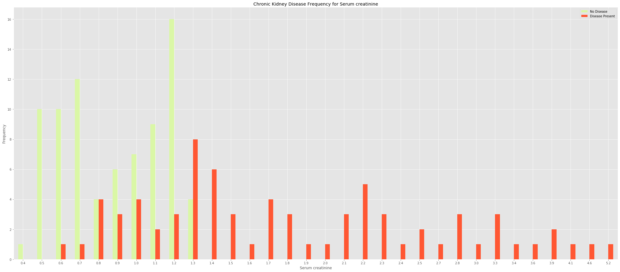
The frequency plot below shows that the lower the serum creatine the less likely you are to have chronic kidney disease. This makes sense as healthy kidneys are known to filter creatinine and other waste products from our blood.

---

The Models

Classification models were tried to check for the best model to predict chronic kidney disease since the prediction of disease versus no disease has a discrete outcome.

• Logistic Regression
• Support Vector Machines
• Linear SVC
• Decision Tree
• Random Forest
• Naive Bayes

5. Methodology

Data Preprocessing

1.Check whether the target data is balanced; i.e. does the patient have chronic kidney disease or not? Initially the target data is skewed toward having chronic kidney disease, 174:106, so some steps were taken to balance it.

1. Fill Yes/No columns with boolean values.
2. Imputing data: Fill the null values with the median value of each column. We didn’t want to lose features like red_blood_cells which was missing 107 out of 280 values, and since the object-type columns were filled with boolean values, the median of each feature column was used instead of the mean.
3. Remove outliers from non-categorical columns: An assumption of binary logistic regression is there should be no outliers in the data so they were identified using the Tukey rule.

def find_outliers(col):
    """
    Identify the outliers of each column of a dataframe using the Tukey rule

    :return: A dataframe of the outliers for each column
    """
    # Calculate the first quartile
    Q1 = df[col].quantile(.25)

    # Calculate the third quartile
    Q3 = df[col].quantile(.75)

    # Calculate the interquartile range Q3 - Q1
    IQR = Q3 - Q1
    IQR

    # Calculate the maximum value and minimum values according to the Tukey rule
    # max_value is Q3 + 1.5 * IQR while min_value is Q1 - 1.5 * IQR

    max_value = Q3 + 1.5 * IQR
    min_value = Q1 - 1.5 * IQR

    # Filter the training data for values that are greater than max_value or less than min_value
    outliers = df[(df[col] > max_value) | (df[col] < min_value)]
    return outliers

1. Using a dataframe with the outliers removed, apply logistic regression and check for class balancing again so there is no chance of one classification being chosen over the other. After using the Tukey rule the classes were balanced slightly more in favour of not having chronic kidney disease: 79:74.

Libraries:

1. numpy
2. pandas
3. matplotlib
4. seaborn
5. sklearn

Each model was coded in a similar way; keeping them simple was the main idea to keep the running time down.

Choice of models

The prediction of disease versus no disease is a classification problem since it has a discrete outcome, so this type of model was investigated for a solution.

Each set of model parameters was tuned using a grid search, and where possible the random state was set for reproducibility.

Logistic Regression: 98.69 percent

Logistic regression makes a great baseline algorithm so this was the starting point in the models. The assumptions made in the feature engineering suit this algorithm. For instance, the dependent variable should be dichotomous in nature (present/absent). In binary logistic regression there should be no outliers in the data. There should also be no high correlations among the predictors.

Logistic regression is probably the most important supervised learning classification method. It’s fast, due to it’s relationship to the generalized linear model, and it works well when the relationship between the features and the target are not too complex. It’s documented on the scikit learn page.

The first working pipeline:

pipeline = Pipeline([
    ('clf', LogisticRegression())
])

parameters = {
    'clf__max_iter': [3000, 4000],
    'clf__fit_intercept': [True, False],
    'clf__penalty': ['l2'],
    'clf__n_jobs': [1,5,8,10],
    'clf__C': [1,5,8],
    'clf__random_state': [34]
}

cv = GridSearchCV(pipeline, param_grid=parameters)

cv.fit(X_train, y_train)
y_pred = cv.predict(X_test)

acc_log_reg = round( clf.score(X_train, y_train) * 100, 2)
print (str(acc_log_reg) + ' percent')

The best parameters were found to be:

cv.best_params_

{‘clf__C’: [0.5], ‘clf__fit_intercept’: False, ‘clf__max_iter’: 3000, ‘clf__n_jobs’: 1, ‘clf__penalty’: ‘l2’, ‘clf__random_state’: 34}

These parameters were tuned because of their impact on regularization. We want to improve the generalization performance; to penalize complexity.

After running the model with the default max_iter’: 100, convergence warnings led to it being increased, and the accuracy in turn improved.

ConvergenceWarning: Liblinear failed to converge, increase the number of iterations.
"the number of iterations.", ConvergenceWarning)

clf__max_iter refers to the maximum number of iterations taken for the solvers (e.g. Liblinear mentioned in the warning) to converge. Increasing clf__max_iter to the 1000s had the greatest impact on accuracy and this turned into the main focus for optimization.

Support Vector Machine: 100 percent

This is a supervised machine learning algorithm (described on scikit-learn) where each data item can be plotted as a point in n-dimensional space (where n is the number of features in the data frame), and the value of each feature is the value of each coordinate. Classification is completed by finding the hyper-plane that differentiates the two classes very well.

The parameters tuned were identified as important as they have the highest impact on this model’s performance: “kernel”, “gamma” and “C”.

pipeline = Pipeline([
    ('standardscaler', StandardScaler()),
    ('clf', SVC())
])

parameters = {
    'clf__C': [0.1, 0.5, 1.0],
    'clf__random_state': [34]
}

cv = GridSearchCV(pipeline, param_grid=parameters)

cv.fit(X_train, y_train)
y_pred_svc = cv.predict(X_test)

Best parameters:

cv.best_params_

{‘clf__C’: 1.0, ‘clf__random_state’: 34} This means that the default parameters worked perfectly! The StandardScaler was used to normalize the training data so that the problem became more conditioned, i.e. transformed the data so its distribution had a mean value 0 and standard deviation of 1; in turn speeding up the convergence. If one feature’s variance is many orders of magnitude more than the variance of other features, that feature would dominate other features in the dataset. The model would not handle this imbalance as we’d need.

Linear SVM: 100 percent

Linear SVM is an SVM model with a linear kernel. LinearSVC stands for Linear Support Vector Classification, and is another (faster) implementation of Support Vector Classification for the case of a linear kernel. More details can be found on scikit-learn.

The StandardScaler was used here again, as discussed in the SVM section above.

Again here the regularization parameter C was found to help with the accuracy. A gridsearch was used as follows:

pipeline = Pipeline([
    ('scaler', StandardScaler()),
    ('clf', LinearSVC())
])

parameters = {
    'clf__C': [0.1, 0.5, 1.0],
    'clf__random_state': [34]
}

cv = GridSearchCV(pipeline, param_grid=parameters)

cv.fit(X_train, y_train)
y_pred_lsvm = cv.predict(X_test)

The best parameters

cv.best_params_

{‘clf__C’: 0.1, ‘clf__random_state’: 34}

Decision Tree: 99.35 percent

Put simply, this model is based on a flowchart-like tree structure where decisions are made at each node of the tree. It is explained on scikit-learn.

The parameters chosen were based on creating a model where each feature is classified correctly for each patient, which is better than randomly choosing the classification.

The min_samples_split is for regularizing the tree, the default is 2 so values were chosen under 10 to ensure the best value was used. The max_depth parameter is one of the ways in which we can regularize the tree, or limit the way it grows to prevent over-fitting.

Pipeline

pipeline = Pipeline([
    ('clf', DecisionTreeClassifier())
])

parameters = {
    'clf__criterion': ['gini', 'entropy'],
    'clf__max_depth': [1, 3, 5, 8, 10],
    'clf__min_samples_split': [2, 3, 5, 8, 10],
    'clf__max_features': ['auto', 'sqrt', 'log2'],
    'clf__random_state': [34]
}

cv = GridSearchCV(pipeline, param_grid=parameters)

cv.fit(X_train, y_train)
y_pred_decision_tree = cv.predict(X_test)

Best parameters:

cv.best_params_

{‘clf__criterion’: ‘gini’, ‘clf__max_depth’: 8, ‘clf__max_features’: ‘auto’, ‘clf__min_samples_split’: 5, ‘clf__random_state’: 34}

Random Forest: 100 percent

The decision tree is the basic building block of a random forest. The random forest is better than a single decision tree because it pools predictions from multiple sources, thereby incorporating much more knowledge than from any one individual. (Described on scikit-learn)

pipeline = Pipeline([
    ('scaler', StandardScaler()),
    ('clf', RandomForestClassifier())
])

parameters = {}

cv = GridSearchCV(pipeline, param_grid=parameters)

cv.fit(X_train, y_train)
y_pred_random_forest = cv.predict(X_test)

Gaussian Naive Bayes: 95.42 percent

Naive Bayes classifiers apply Bayes’ theorem with strong independence assumptions between the features. The Gaussian Naive Bayes algorithm (described on scikit-learn) assumes a Gaussian (normal) distribution, and takes just two parameters: clf__priors parameter to specify weighted probabilities for classes and clf__var_smoothing (categorical variable smoothing).

pipeline = Pipeline([
    ('clf', GaussianNB())
])

parameters = {
    'clf__priors': [None],
    'clf__var_smoothing': [0.00000001, 0.000000001, 0.00000001]
}

cv = GridSearchCV(pipeline, param_grid=parameters)

cv.fit(X_train, y_train)
y_pred_gnb = cv.predict(X_test)

Best parameters

cv.best_params_

{‘clf__priors’: None, ‘clf__var_smoothing’: 1e-08}

Refinement

The following section explains the improvements made to some of the models.

The logistic regression model was refined by removing most of the parameters from the grid search. Adding more parameters did not improve on the model’s accuracy. Instead of using the parameters

parameters = {
    'clf__max_iter': [3000, 4000],
    'clf__fit_intercept': [True, False],
    'clf__penalty': ['l2'],
    'clf__n_jobs': [1,5,8,10],
    'clf__C': [1,5,8],
    'clf__random_state': [34]
}

the following could be used for the same result:

parameters = {
    'clf__max_iter': [3000],
    'clf__random_state': [34]
}

Hence the runtime was improved.

The Linear SVM model was also improved significantly from 51.63 to 100 percent when the standard scaler was added to the pipeline. The StandardScaler was used to normalize the training data so that no feature would dominate other features in the dataset. The model would not handle this imbalance as we would require, hence the big jump in accuracy.

pipeline = Pipeline([
    ('scaler', StandardScaler()),
    ('clf', LinearSVC())
])

parameters = {
    'clf__C': [0.1, 0.5, 1.0],
    'clf__random_state': [34]
}

Both the Decision Tree and Random Forest classifier improved from 99.35 to 100 perecent by resorting to the default values.

Decision Tree

parameters = {'clf__criterion': 'gini',
 'clf__max_depth': 8,
 'clf__max_features': 'auto',
 'clf__min_samples_split': 5,
 'clf__random_state': 34}

Default: parameters = {}

Random Forest

parameters = {
    'clf__n_estimators': [50, 100, 200],
    'clf__criterion': ['gini', 'entropy'],
    'clf__max_depth': [1, 3, 5, 8, 10],
    'clf__min_samples_split': [2, 3, 5, 8, 10],
    'clf__max_features': ['auto', 'sqrt', 'log2'],
    'clf__random_state': [34]
}

Default: parameters = {}

6. Results

Model Evaluation and Validation

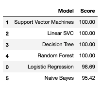
In this investigation starting with the default values has worked out best in creating classification models to predict chronic kidney disease. Four out of six models reached 100% accuracy.

Below is a table ranking the models applied to the data according to the scores they produced. We can see that Decision Tree and Random Forest classfiers have the highest accuracy score. This similarity makes sense as random forests are an example of an ensemble learner built on decision trees.

Between these two, the Random Forest classifier is a better choice as it has the ability to limit overfitting when compared to the Decision Tree classifier.

---

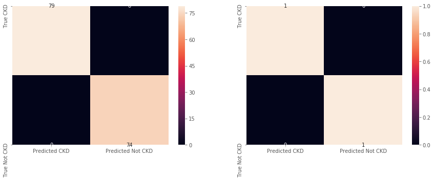
Chronic kidney disease can be predicted 100% from the provided dataset using the SVM, Random Forest, Linear SVC, and the Decision Tree classifiers. It’s confusion matrix is shown below.

Justification

At scale, with more data, the Random Forest classfier would be my first choice in predicting chronic kidney disease as it belongs to the family of ensemble methods which help improve machine learning results by combining multiple models. Using ensemble methods produces better predictions compared to a single model, hence they have a history of placing first in many prestigious machine learning competitions on Kaggle.

7. Conclusion

Real-world context

When a woman who has had preeclampsia presents herself to medical staff after pregnancy and she has her blood drawn due to symptoms related to preeclampsia/eclampsia, the features used in this dataset can be taken from her blood and used to determine whether or not she has chronic kidney disease.

Chronic kidney disease can be predicted 100% from the provided dataset using the Random Forest Classifier. The feature most correlated to this prediction is serum creatinine, which makes sense as healthy kidneys are known to filter creatinine and other waste products from our blood.

Reflections

The SVM, Random Forest, Linear SVC, and the Decision Tree classifiers performed best in the group of models used to predict chronic kidney disease from patient data.

Removing the outliers needed some reflection as a few variables were categorical and it did not make sense to remove some of those categories. Some careful consideration was required for these variables and it paid off in the performance of the logistic regression. However, in the end, that was not the best model as it was expected to be. The Random Forest classifier was best due to it’s ability to limit overfitting as an ensemble method.

Improvements

There was not much open data found for kidney disease, but if it was found in abundance then the chosen model may change due to considerations of performance time, and more parameters would be tested to ensure the performance was optimal.

---

7. Licensing, Authors, Acknowledgements

The data files were retrieved from Kaggle, via UCI.

Thanks to Udacity for supporting this project.